PWR Accumulator Modeling¶

Overview¶

This section provides guidance on how to model a typical PWR accumulator and its discharge line in TRACE. The guidance applies to the following commercial PWR designs:

Westinghouse 2-loop PWR
Westinghouse 3-loop PWR
Westinghouse 4-loop PWR
Combustion Engineering 2-loop PWR
Babcock and Wilcox PWR

The guidance is written assuming the analyst is building the model in SNAP, but the corresponding ASCII input variable names are also referenced.

Source

This page is extracted from TRACE PWR Modeling Guidance, Revision 1 (February 2015), Section 12 — PWR Accumulator Modeling Guidance and Appendix A.12 — Accumulators.

Component Function¶

The accumulator is a passive ECCS component. It contains borated water held under pressure by a non-condensable gas cushion (typically nitrogen) and discharges automatically through a check valve when primary system pressure drops below the accumulator gas pressure — as during a LOCA.

Required Inputs¶

Before building the model, obtain the following plant-specific information:

Required Plant Data Checklist

Component Selection¶

System Element	TRACE Component	Rationale
Accumulator tank	PIPE (PIPETYPE `IACC = 2`)	Non-spherical accumulator with interface sharpener and level tracking
Discharge line with check valve	VALVE (`IVTY = 9`, check valve)	Allows flow-area-controlled discharge on reverse ΔP

Why IACC = 2?

TRACE provides specialized PIPE types for accumulators. PIPETYPE = 2 includes a specialized discharge model for non-spherical accumulators, an interface sharpener at the accumulator exit, and a level-tracking model that prevents gaseous discharge until all liquid is gone. Because the level-tracking model requires the second junction (PIPE outlet) to be the accumulator outlet, the tank is oriented downward (gas at the top, discharge at the bottom).

Accumulator PIPE Component¶

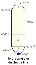
A typical accumulator PIPE has 6 cells and 7 edges.

Figure 12.2-1 — Typical accumulator nodalization.

Component Initialization (SNAP)¶

Input	Value
Total Length	Accumulator height (\(H_{accum}\))
Hydraulic Diameter (HD)	Accumulator diameter (overwritten per edge below)
Number of Cells (NCELLS)	6
Number of Pipes (NPIPES)	1
Orientation	Vertical

Naming conventions:

Component Name (CTITLE): Loop # - Accumulator — or Loop # - Accumulator A/B for plants with two accumulators per loop.
Component Number (NUM): (Loop number) * 100 + 1040 (single or Accumulator A); (Loop number) * 100 + 1070 (Accumulator B).
Description: Reference the source of the design information.

Geometry Inputs¶

The guidance assumes the accumulator tank is cylindrical with hemispherical caps on top and bottom. In SNAP, select the "Area" radio button on the Cells tab so that SNAP calculates the volume-averaged flow area while the analyst enters cell volumes, lengths, and the edge flow areas separately.

Cell Length (DX)¶

\[ \begin{aligned} DX_{cell\,1} &= IR_{hemisphere} \\ DX_{cells\,2,3,4} &= \frac{H_{accum} - 2 \, IR_{hemisphere}}{3} \\ DX_{cells\,5,6} &= \frac{IR_{hemisphere}}{2} \end{aligned} \]

Cell Volume (VOL)¶

If detailed tank geometry is available, compute exact per-cell volumes. Otherwise use the closed-form expressions below (cylinder with hemispherical caps). Verify the cell volumes sum to the total accumulator volume and adjust as needed.

\[ \begin{aligned} VOL_{cell\,1} &= \tfrac{2}{3}\pi \, IR_{hemisphere}^{3} \quad \text{(hemisphere)} \\ VOL_{cells\,2,3,4} &= \pi \, IR_{cylinder}^{2} \, DX_{cells\,2,3,4} \\ VOL_{cell\,5} &= VOL_{cell\,1} - VOL_{cell\,6} \\ VOL_{cell\,6} &= \tfrac{\pi \, DX_{cell\,6}}{6}\left(3\,IR_{hemisphere}^{2} - 2\,DX_{cell\,6}^{2}\right) \quad \text{(spherical cap)} \end{aligned} \]

10:1 Volume Ratio Check

After computing cell volumes, verify that adjacent-cell volumes do not exceed the 10:1 volume-ratio guidance. If they do, adjust DX values accordingly. Also compare the SNAP-computed volume-averaged FA to the analyst-computed edge FA for cells with no flow-area change — they should be approximately equal.

Edge Flow Area (FA)¶

\[ \begin{aligned} FA_{edge\,1} &= 0.0 \\ FA_{edges\,2,3,4,5} &= \frac{\pi \, ID_{cylinder}^{2}}{4} \\ FA_{edge\,6} &= \pi \left(IR_{hemisphere}^{2} - DX_{cell\,6}^{2}\right) \\ FA_{edge\,7} &= \frac{\pi \, ID_{AccumDischargeLine}^{2}}{4} \end{aligned} \]

Edge Hydraulic Diameter (HD)¶

Do not select "Calculate Hydraulic Diam." in SNAP — enter these values explicitly.

\[ \begin{aligned} HD_{edge\,1} &= 1.0 \times 10^{10} \quad \text{(TRACE requires HD > 0)} \\ HD_{edges\,2,3,4,5} &= ID_{cylinder} \\ HD_{edge\,6} &= 2\sqrt{IR_{hemisphere}^{2} - DX_{cell\,6}^{2}} \\ HD_{edge\,7} &= ID_{AccumDischargeLine} \end{aligned} \]

Edge CCFL Model¶

CCFL is not expected in the accumulator. Do not activate the CCFL model:

\[LCCFL_{edges\,1-7} = 0\]

Orientation, Angle (θ), and GRAV¶

The accumulator is vertical. If plant-specific orientation information is available, use it; otherwise use the typical PWR values:

Parameter	Value (edges 1–7)
Orientation	Vertical
Angle \(\theta\)	\(-1.571\) rad
GRAV = \(\sin\theta\)	\(-1.0\)

Initial Conditions¶

Accumulator ICs should be a reasonable estimate of plant steady-state conditions. The steady-state run will refine the values used to initialize the transient.

Thermodynamic Consistency

Initial pressures and temperatures must be thermodynamically consistent.

Cell ICs¶

Variable	Value
\(P_{cells\,1-6}\)	Nominal accumulator pressure
\(TL_{cells\,1-6}\)	Nominal accumulator water temperature
\(TV_{cells\,1-6}\)	Nominal accumulator water temperature

Gas Volume Fraction (ALPN) — Transition Cell Method¶

The "transition cell" (cell \(t\)) is the cell containing the liquid–gas interface. Cells below \(t\) are all liquid; cells above \(t\) are all gas.

Locate the transition cell:
- If \(VOL_{AccumWater} < VOL_{cell\,6}\), then \(t = 6\).
- If \(VOL_{cell\,6} < VOL_{AccumWater} < VOL_{cell\,6} + VOL_{cell\,5}\), then \(t = 5\).
- If \(VOL_{AccumWater} > VOL_{cell\,6} + VOL_{cell\,5}\), compute the transition height from the bottom of the tank:
\[ H_{transition} = IR + \frac{VOL_{AccumWater} - \tfrac{2}{3}\pi \, IR^{3}}{\pi \, IR^{2}} \]
Then set:

\[ \begin{aligned} ALPN_{cells\,1\,\ldots\,(t-1)} &= 1.0 \\ ALPN_{cell\,t} &= 1 - \frac{VOL_{AccumWater} - VOL_{cells\,(t+1)\,\ldots\,6}}{VOL_{cell\,t}} \\ ALPN_{cells\,(t+1)\,\ldots\,6} &= 0.0 \end{aligned} \]

Non-Condensable Partial Pressure (PA)¶

\[ \begin{aligned} PA_{cell\,1\,\ldots\,t} &= P_{nominal} - P_{sat}(T_{water}) \\ PA_{cell\,(t+1)\,\ldots\,6} &= 0.0 \end{aligned} \]

Edge ICs¶

Accumulator flow is zero at steady state:

\[VL_{edges\,1-7} = VV_{edges\,1-7} = 0.0\]

Friction Inputs¶

Friction Factor Correlation (NFF)¶

Nodalization Criterion

Section 1.5 of the Rev 1 guidance defines a nodalization criterion that must be checked for cells adjacent to edges where NFF = 0. For the accumulator, verify the cells adjacent to edge 7.

\[ \begin{aligned} NFF_{edges\,1,2} &= 0 \\ NFF_{edges\,3,4} &= 1 \\ NFF_{edges\,5,6,7} &= 0 \end{aligned} \]

Forward Loss Coefficient (KFAC)¶

KFAC is only modeled at edges where flow area or direction changes. A small non-zero placeholder (1.0E-10) is entered at a few edges with area changes that are already accounted for at edge 7 — this suppresses a SNAP/TRACE warning for the unaccounted area change.

\[ \begin{aligned} KFAC_{edges\,1,3,4} &= 0.0 \\ KFAC_{edges\,2,5,6} &= 1.0 \times 10^{-10} \\ KFAC_{edge\,7} &= 0.5\,(1 - \beta^{2}) \quad \text{(sudden contraction)} \\ \text{where } \beta &= \frac{ID_{AccumDischargeLine}}{ID_{Accumulator}} \end{aligned} \]

Reference: Crane TP-410 (Reference 4 in the Rev 1 guide), page 2-11.

Reverse Loss Coefficient (KFACR)¶

\[ \begin{aligned} KFACR_{edges\,1,3,4} &= 0.0 \\ KFACR_{edges\,2,5,6} &= 1.0 \times 10^{-10} \\ KFACR_{edge\,7} &= (1 - \beta^{2})^{2} \quad \text{(sudden expansion)} \end{aligned} \]

Choked Flow Model (ICFLG)¶

Choked flow is not expected within the accumulator:

\[ICFLG_{edges\,1-7} = 0\]

General Inputs¶

Input	SNAP setting / Value	Notes
Solute in coolant (`ICONC`)	Per Section 1.6	—
Initial boron concentration (`CONC`)	Nominal tank value (ppm)	If `ICONC = 1`
Fluid power option (`IPOW`)	`0` (Not modeled)	No direct fluid power in the tank
Wall roughness (`EPSW`)	Plant value, or \(4.572 \times 10^{-5}\) m (1.5E-4 ft) for commercial steel	—
Cross-flow connections (`NSIDES`)	`0`	No side junctions
PIPETYPE (`IACC`)	`2`	Non-spherical accumulator with level tracking
Leak paths	`0`	Do not use TRACE internally spawned leak paths
Pipe wall & wall power	Per Section 1.7	—

Accumulator Discharge Line (VALVE Component)¶

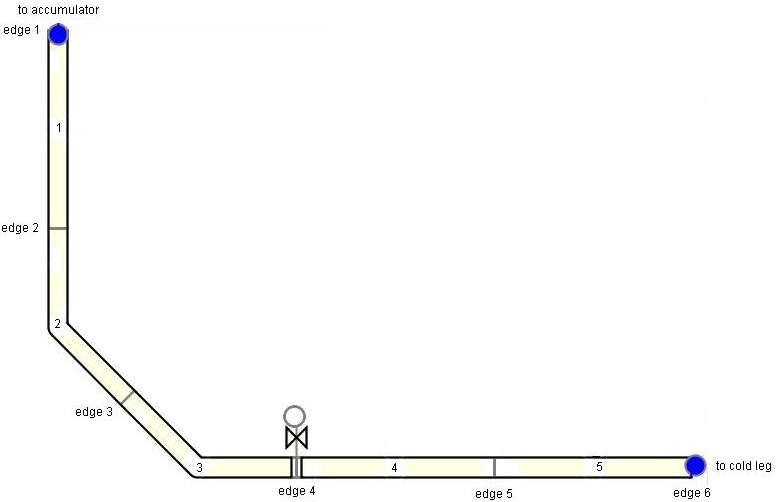
A typical discharge-line VALVE has 5 cells and 6 edges. The nodalization is generic; if the plant geometry differs significantly, adjust the DX and orientation to represent the actual pipe bends.

Figure 12.2-2 — Typical accumulator discharge line nodalization.

Component Initialization (SNAP)¶

Input	Value
Total Length	Discharge line length
Hydraulic Diameter (HD)	\(ID_{AccumDischargeLine}\)
Number of Cells (NCELLS)	5
Orientation	Horizontal

Naming conventions:

Component Name: Loop # - Accumulator Discharge Line — or suffix A/B as appropriate.
Component Number: (Loop number) * 100 + 1045 (single / A); (Loop number) * 100 + 1075 (B).

Geometry Inputs¶

Cell Length / Volume¶

Five equal-length cells covering the entire line from accumulator exit to cold leg entrance. Adjust lengths as needed to place elbows and the check valve appropriately.

\[ \begin{aligned} DX_{cells\,1-5} &= \frac{L_{AccumDischargeLine}}{5} \\ VOL_{cells\,1-5} &= \pi \, IR_{AccumDischargeLine}^{2} \, DX_{cells\,1-5} \end{aligned} \]

Check the 10:1 volume-ratio guidance as before.

Edge Flow Area (FA)¶

\[ \begin{aligned} FA_{edges\,1,2,3,5,6} &= \frac{\pi \, ID_{AccumDischargeLine}^{2}}{4} \\ FA_{edge\,4} &= \frac{\pi \, ID_{AccumCheckValveFullyOpened}^{2}}{4} \end{aligned} \]

Edge Hydraulic Diameter (HD)¶

\[ \begin{aligned} HD_{edges\,1,2,3,5,6} &= ID_{AccumDischargeLine} \\ HD_{edge\,4} &= ID_{AccumCheckValveFullyOpened} \end{aligned} \]

CCFL¶

\[LCCFL_{edges\,1-6} = 0\]

Orientation, Angle, and GRAV¶

Edges	Orientation	Angle (rad)	GRAV
1, 2	Vertical	\(-1.571\)	\(-1.0\)
3	Angled (−45°)	\(-0.7855\)	\(-0.707\)
4, 5, 6	Horizontal	\(0.0\)	\(0.0\)

Initial Conditions¶

Cell ICs¶

Variable	Cells 1–3	Cells 4–5
Pressure (`P`)	Nominal accumulator pressure	Plant-specific SS pressure, else primary system nominal
Liquid temp (`TL`)	Nominal accumulator water temperature	Plant-specific SS temperature, else RV inlet temperature
Vapor temp (`TV`)	Nominal accumulator water temperature	Plant-specific SS temperature, else RV inlet temperature
Gas volume fraction (`ALPN`)	0.0	0.0
Non-condensable partial pressure (`PA`)	0.0	0.0

Edge velocities are zero at steady state:

\[VL_{edges\,1-6} = VV_{edges\,1-6} = 0.0\]

Friction Inputs¶

Nodalization Criterion

Check the cells adjacent to edges 1 and 6 against the nodalization criterion in Section 1.5 because these edges use NFF = 0.

\[ \begin{aligned} NFF_{edges\,1,6} &= 0 \\ NFF_{edges\,2-5} &= 1 \end{aligned} \]

Check-Valve Edge Special Case

If the valve's fully-opened flow area is much smaller than the pipe area (\(FA_{pipe} > 2 \, FA_{valve}\)), set \(NFF_{edge\,4} = 0\) and add an appropriate \(KFAC\) / \(KFACR\) at edge 4. This is not expected in typical designs but should be checked.

Loss Coefficients¶

Loss coefficients are modeled at edges 1 (contraction from accumulator), 3 (pipe bends), 4 (check valve), and 6 (expansion into cold leg).

Define \(\beta_{1} = ID_{AccumDischargeLine} / ID_{Accumulator}\) and \(\beta_{6} = ID_{AccumDischargeLine} / ID_{ColdLeg}\). The Darcy friction factor \(f_{T}\) is taken from the smooth-commercial-steel-pipe table in Crane TP-410 (Reference 4).

Edge	Feature	KFAC (forward)	KFACR (reverse)
1	Contraction from tank	\(0.5\,(1-\beta_{1}^{2})\)	\((1-\beta_{1}^{2})^{2}\)
2	Straight pipe	0.0	0.0
3	Two 45° elbows	\(32\,f_{T}\)	\(32\,f_{T}\)
4	Swing check valve	\(50\,f_{T}\)	\(50\,f_{T}\)
5	Straight pipe	0.0	0.0
6	Expansion into cold leg	\((1-\beta_{6}^{2})^{2}\)	\(0.5\,(1-\beta_{6}^{2})\)

Bend Loss Coefficients

The edge-3 value of \(32\,f_{T}\) represents two 45° standard elbows (\(2 \times 16\,f_{T}\)). For other bend angles, derive the appropriate coefficient — for example, a 90° standard elbow is \(30\,f_{T}\).

TRACE will automatically apply an adjusted loss coefficient across the valve edge to account for the valve flow-area fraction (per Equation 2-127 of the Theory Manual) when INTLOSSOFF = 0.

Choked Flow Model (ICFLG)¶

Choking is only expected at the discharge-line exit into the cold leg:

\[ \begin{aligned} ICFLG_{edges\,1-5} &= 0 \\ ICFLG_{edge\,6} &= 1 \end{aligned} \]

General and Valve Inputs¶

Input	Value	Notes
Solute in coolant (`ICONC`)	Per Section 1.6	—
Initial boron (`CONC`), cells 1–3	Nominal accumulator value (ppm)	—
Initial boron (`CONC`), cells 4–5	Primary system nominal (ppm)	—
Valve type (`IVTY`)	`9` — Check Valve	—
Fluid power (`IPOW`)	`0`	Not modeled
Wall roughness (`EPSW`)	\(4.572 \times 10^{-5}\) m if unknown	—
Valve interface edge (`IVPS`)	Edge 4 of 6	Valve flow area adjusted here
Flow-area adjustment type (`IVTYOV`)	`0` — Flow Area Fraction / sec	—
Internal loss model (`INTLOSSOFF`)	`0` — On	See rationale below
Max valve rate (`RVMX`)	\(1 / t_{open/close}\)	—
Off-adjustment rate (`RVOV`)	\(1 / t_{open/close}\)	—
Min/max position (`FMINOV` / `FMAXOV`)	0.0 / 1.0	Fully closed / fully open
Valve flow area (`AVLVE`)	Fully-opened check-valve flow area	—
Valve hydraulic diameter (`HVLVE`)	Fully-opened check-valve HD	—
Initial valve fraction (`FAVLVE`)	0.0	Check valves start closed
Initial stem position (`XPOS`)	0.0	Consistent with `FAVLVE`
Check-valve type (`HYSTER`)	`0` — Static Pressure / Flow with Hysteresis	—
Open delta pressure (`ADDDP`)	Spring-loading ΔP of the plant valve	—
Leak area ratio (`LEAKARAT`)	Leak area / open area (or 0 if none)	—
Latch option (`LATCHOPT`)	`0` — Open/Close Repeatedly	Required for reclosure behavior
Leak paths	`0`	No TRACE internally spawned leak paths
Signal variable (`IVSV`)	`0`	Not used for check valves
Override trip (`IVTROV`)	`0`	Not used for check valves
Pipe wall & wall power	Per Section 1.7	—

Why the Internal Loss Model is Used Here

For most PWR valves, TRACE's internal additive flow-loss model is not used because manufacturer-tested loss coefficients are readily available. Accumulator check valves are an exception: they operate across a wide range of conditions and flapper positions, so their loss coefficients are more uncertain. NRC staff engineering judgment is to apply the internal loss model here to correct for the unknowns.

Geometry Input Summary¶

Accumulator PIPE (Table 12.5-1)¶

Node	DX	VOL	Edge	FA	HD	GRAV	KFAC	KFACR	NFF
1	\(IR_{hemi}\)	\(\tfrac{2}{3}\pi IR^{3}_{hemi}\)	1	0.0	\(1.0 \times 10^{10}\) †	−1.0	0.0	0.0	0
2	\((H_{accu}-2IR_{hemi})/3\)	\(DX_{2}\cdot FA_{2}\)	2	\(\pi ID_{2}^{2}/4\)	pipe \(ID_{2}\)	−1.0	1.0E-10	1.0E-10	0
3	\((H_{accu}-2IR_{hemi})/3\)	\(DX_{3}\cdot FA_{3}\)	3	\(\pi ID_{3}^{2}/4\)	pipe \(ID_{3}\)	−1.0	0.0	0.0	1
4	\((H_{accu}-2IR_{hemi})/3\)	\(DX_{4}\cdot FA_{4}\)	4	\(\pi ID_{4}^{2}/4\)	pipe \(ID_{4}\)	−1.0	0.0	0.0	1
5	\(IR_{hemi}/2\)	\(VOL_{1}-VOL_{6}\)	5	\(\pi ID_{5}^{2}/4\)	pipe \(ID_{5}\)	−1.0	1.0E-10	1.0E-10	0
6	\(IR_{hemi}/2\)	\(\tfrac{\pi DX_{6}}{6}(3IR^{2}_{hemi}-2DX^{2}_{6})\)	6	\(\pi(IR^{2}_{hemi}-DX^{2}_{6})\)	\(2\sqrt{IR^{2}_{hemi}-DX^{2}_{6}}\)	−1.0	1.0E-10	1.0E-10	0
			7	\(\pi ID^{2}_{acculine}/4\)	\(ID_{7}\) discharge line	−1.0	\(0.5(1-\beta^{2})\)	\((1-\beta^{2})^{2}\)	0

\(EPSW\) = known value, else \(4.572 \times 10^{-5}\) m. \(\beta = ID_{edge\,7} / ID_{edge\,5}\). CCFL not activated on any edge. † TRACE requires HD > 0.

Accumulator Discharge Line VALVE (Table 12.5-2)¶

Node	DX	VOL	Edge	FA	HD	GRAV	KFAC	KFACR	NFF	ICFLG
1	\(L_{tot}/5\)	\(DX_{1}\cdot FA_{1}\)	1	\(\pi ID_{1}^{2}/4\)	pipe \(ID_{1}\)	−1.0	\(0.5(1-\beta_{1}^{2})\)	\((1-\beta_{1}^{2})^{2}\)	0	0
2	\(L_{tot}/5\)	\(DX_{2}\cdot FA_{2}\)	2	\(\pi ID_{2}^{2}/4\)	pipe \(ID_{2}\)	−1.0	0.0	0.0	1	0
3	\(L_{tot}/5\)	\(DX_{3}\cdot FA_{3}\)	3	\(\pi ID_{3}^{2}/4\)	pipe \(ID_{3}\)	\(\sin(-45°)\)	\(32 f_{T}\)	\(32 f_{T}\)	1	0
4	\(L_{tot}/5\)	\(DX_{4}\cdot FA_{5}\)	4 (check valve ‡)	\(\pi ID^{2}_{openvalve}/4\)	\(ID_{4}\) fully open	0.0	\(50 f_{T}\) ‡‡	\(50 f_{T}\) ‡‡	1 ‡‡	0
5	\(L_{tot}/5\)	\(DX_{5}\cdot FA_{5}\)	5	\(\pi ID_{5}^{2}/4\)	pipe \(ID_{5}\)	0.0	0.0	0.0	1	0
			6	\(\pi ID_{6}^{2}/4\)	pipe \(ID_{6}\)	0.0	\((1-\beta_{6}^{2})^{2}\)	\(0.5(1-\beta_{6}^{2})\)	0	1

\(\beta_{1} = ID_{edge\,1} / ID_{Accumulator}\). \(\beta_{6} = ID_{edge\,6} / ID_{ColdLeg}\). \(L_{tot}\) = discharge line total length. \(f_{T}\) is from Table 1.5-1 of the Rev 1 guide. ‡ IVTY = 9; see valve inputs above. ‡‡ If \(FA_{pipe} > 2 \, FA_{valve}\), set \(NFF_{edge\,4} = 0\) and add appropriate \(KFAC/KFACR\) at edge 4.

Steady-State Initialization Criteria¶

For model-to-plant comparisons during steady-state initialization, the Rev 1 guidance (Section 29.x, PWR Steady-State Initialization) recommends the following tolerances for accumulator parameters:

Parameter	Acceptance Criterion
Accumulator liquid temperature	Target Value ± 0.007 MPa (1 psi equivalent)
Accumulator pressure	Target Value ± 1 K (1.8 °F)
Accumulator liquid level	Target Value ± 1%

Modeling Basis (Appendix A.12)¶

The rationale behind the recommended approach:

Why this nodalization

TRACE provides specialized accumulator PIPE types; PIPETYPE = 2 is recommended because it includes specialized discharge models for non-spherical accumulators, an interface sharpener at the exit, and a level-tracking model that prevents gaseous discharge until all liquid is gone. The level-tracking model requires the second junction (PIPE outlet) to be the accumulator outlet — so the tank is oriented downward.

The tank is modeled as a cylinder with hemispherical caps. The nodalization was developed from LOCA-analysis modeling experience to adequately capture the key thermal-hydraulic phenomena documented in the applicable PIRTs, without unnecessary increase in computational cost. The tank is connected via a conical-frustum nozzle to the discharge line, which is a simple cylindrical pipe with several bends and a check valve. Because exact bend geometry varies by plant, the analyst is responsible for verifying the actual configuration.

Non-condensable gas

Accumulators typically contain nitrogen to pressurize the liquid. The gas can be specified as nitrogen (Section 1, subsection 1), but modeling experience has shown that TRACE's default non-condensable (air) is an adequate substitute in most analyses. When deciding whether to change to nitrogen, consider the presence of other non-condensable gases in the system — especially in any CONTAN components in the model.

Why the internal loss model is applied to the check valve

TRACE's internal additive loss model is not typically used for PWR valves because manufacturer-tested loss coefficients are readily available. Accumulator check valves are an exception: they operate across a wide range of conditions and flapper positions, so the appropriate loss coefficient is more uncertain. It is NRC staff engineering judgment that applying the internal loss model is appropriate here.

Check-valve placement

The check valve is deliberately placed at edge 4 (rather than immediately adjacent to the cold leg) to help reduce chattering and associated numerical problems. Check-valve operation is controlled by the pressure difference between the volumes adjacent to the valve edge, and pressure fluctuations are more likely on the cold-leg side — so the valve is positioned so that the adjacent volume is "insulated" from the cold leg by one additional cell. Recent versions of TRACE have improved check-valve stability, which may allow relocation of the valve for specific applications if there is a justifiable reason; absent a compelling reason, follow the recommended placement.

See Appendix A.23 of the Rev 1 guide for further discussion generic to all thermal-hydraulic components.

References¶

TRACE PWR Modeling Guidance, Revision 1, U.S. NRC, February 2015 — Section 12 and Appendix A.12.
TRACE V5.0 Theory Manual, U.S. NRC, ADAMS ML120060218 — Equation 2-127 (internal valve loss model).
TRACE V5.0 User's Manual, Volume 2: Modeling Guidelines, U.S. NRC, ADAMS ML120060402.
Crane Technical Paper No. 410, Flow of Fluids Through Valves, Fittings, and Pipe (loss-coefficient tables for sudden contractions/expansions, elbows, and check valves).

Extracted from TRACE PWR Modeling Guidance, Rev 1 (Feb 2015), §12 and App. A.12. No discrepancies were found between the PDF and the corresponding component-level Word source (Historical-Rev_1/Accum.docx).

PWR Accumulator Modeling¶

Overview¶

Component Function¶

Required Inputs¶

Component Selection¶

Accumulator PIPE Component¶

Component Initialization (SNAP)¶

Geometry Inputs¶

Cell Length (DX)¶

Cell Volume (VOL)¶

Edge Flow Area (FA)¶

Edge Hydraulic Diameter (HD)¶

Edge CCFL Model¶

Orientation, Angle (θ), and GRAV¶

Initial Conditions¶

Cell ICs¶

Gas Volume Fraction (ALPN) — Transition Cell Method¶

Non-Condensable Partial Pressure (PA)¶

Edge ICs¶

Friction Inputs¶

Friction Factor Correlation (NFF)¶

Forward Loss Coefficient (KFAC)¶

Reverse Loss Coefficient (KFACR)¶

Choked Flow Model (ICFLG)¶

General Inputs¶

Accumulator Discharge Line (VALVE Component)¶

Component Initialization (SNAP)¶

Geometry Inputs¶

Cell Length / Volume¶

Edge Flow Area (FA)¶

Edge Hydraulic Diameter (HD)¶

CCFL¶

Orientation, Angle, and GRAV¶

Initial Conditions¶

Cell ICs¶

Friction Inputs¶

Loss Coefficients¶

Choked Flow Model (ICFLG)¶

General and Valve Inputs¶

Geometry Input Summary¶

Accumulator PIPE (Table 12.5-1)¶

Accumulator Discharge Line VALVE (Table 12.5-2)¶

Steady-State Initialization Criteria¶

Modeling Basis (Appendix A.12)¶

References¶

Related Topics¶